Home Science Page Data Stream Momentum Directionals Root Beings The Experiment
Within the simple Seed Equation are the instructions for unfolding our structure. Just as a seed unfolds into a tree or plant, this equation unfolds into a bigger equation, a Raveled and Furled Equation. Unraveling the Equation is no big thing. (Maybe Raveling is an unnecessary middle step. It could have easily been bundled up with Furling, but we wanted to look at the Furling/Unfurling operation all by itself.) But it is a big deal to Unfurl our Unfolded, Unraveled Equation. This section looks at a few reasons why.
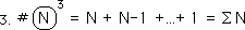
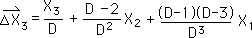
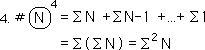
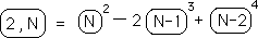
In the Root & Seed Notebook, we derived a seed equation, which had to first be unfolded. After the unfolding, we were left with terms that need to be unraveled and unfurled, in order to determine any of the directionals. Even for the 2nd Directional, shown below, a double, triple, and quadruple unraveling are necessary to determine specific values. The current study is to determine how many terms there are in each unraveling.
The number of terms in a single unraveling is, of course, 1, because it is the data itself. It is already unraveled.
For a double unraveling the number of terms is N, because each piece of Data is necessary in determining the Decaying Average, which is a double unraveling or the data unfurled once divided by D.
For a triple unraveling, the number of terms increases significantly. It is the sum of all the integers from 1 to N.
Let us mention at this point that there are still only N data points needed. If all the terms are combined then there are only N terms. However, the coefficient of each term increases in complexity with each additional unraveling. (See the terms below for an elementary directional.)
For a quadruple unraveling, which is necessary for the 2nd Directional, the number of terms is equal to the sum of all the integers from 1 to N, plus the sum of all the integers from 1 to N-1, plus and so forth down to one. The number of terms is incredible, with a subsequent increase in the complexity of the coefficients of the individual terms.
The pattern is easy to see. Below is the general expression. It is easy to see that when N is even moderately large that the number of terms is out of control for even the simplest directional.
Before proceeding any further, we would like to hammer on the content-based approach for individual derivatives in Living Data Streams. While the Seed Equation is simplicity itself, to make practical use of it requires so many unfoldings, unravelings and unfurlings, that the number of terms to be dealt is prohibitive. With the contextual based approach, only a handful of terms need be stored to find even the current 4th directional after 100 data points. With the content-based approach, 100 terms need to be stored to even calculate the Decaying Average, the zeroth directional.
We have beat upon the content-based approach to individual derivatives enough. We are going to let it go now. We are now going to look at some marvelous implications of the content-based approach on general levels. While the contextual approach is superior for individual derivatives, the content-based approach is superior to discover general characteristics of the foundations of the derivative approach to Live Data Streams. The content-based approach helps us understand the Nature of Derivatives, while the contextual approach helps us calculate the Derivatives, and give the individual derivatives meaning in the context of their occurrence. Meaning vs. Nature
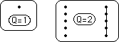
Below are some diagrams of the number of elements in each Unraveling. When Q = 1, from Equation #5 above, we have a point, zero dimensions. When Q = 2 and N = 5, we have a series of 5 points, which we will connect in a line, 1 dimension.
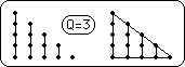
In the third level of Unraveling, when Q = 3 and N = 5, we have a series of 5, 4, 3, 2, & 1 points. First we connect them into lines. Then we connect these lines into a 2 dimensional area. This area is a right triangle.
In the fourth level of Unraveling, when Q = 4 and N = 5, we have a series of 5, 4, 3, 2, & 1 points, plus a series of 4, 3, 2, & 1 points, plus a series of 3, 2, & 1 points, plus a series of 2 & 1 points, plus a series of 1 point. First we connect them into lines, then we connect these lines into triangles, finally we connect the triangles into a solid, 3 dimensions. This solid is a right triangular prism.
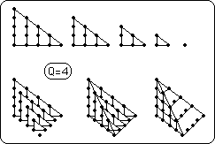
In the fifth level of Unraveling, when Q = 5 and N = 5, we have a solid, a right triangular prism of altitude & base 5, plus a similar prism with height and base of 4, also one of 3, & 2, & 1. If we could we would nest these solids within each other to suggest a four dimensional object. Instead we'll just show the solids.
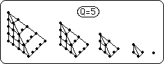
In the sixth level of Unraveling, when Q = 6 and N = 5, we have a series of 5 four-dimensional objects, which we will show broken into their nested solids, right triangular prisms. If we could we would nest these four dimensional object within each other to suggest a five dimensional object. Instead we'll just show the solids. It is easy to get the idea. With each level of unraveling comes another level of dimensionality.

Remember, however, that raveling and dimensionality are only connected in the construction of the individual directionals. If there are other connections, they are indirect. Here we are only discovering the number of elements in each unraveling and have found out that a dimensional analogy helps to visualize the rapid growth of elements in each Raveling
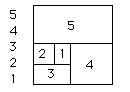
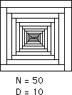
We must also remember that although the number of points is 5, that their potential impact on the derivative is not equal, but varies according their proximity to the derivative. The below Diagram gives a sketch of their potential impact upon the zeroth derivative, the Decaying Average. It spirals inward, diminishing in impact with each successive layer.
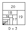
With 20 Data points and a D of 3, we get the diagram below. Notice how the most recent data point, 20, represents a third of the potential impact while the other 19 points represent the remaining two thirds.
When D = 10, the most recent Data represents only 10% of the impact, while the rest of the Data added up yields 90% of the impact. The density of the Data Derivatives increases as D increases. D can only increase when N is sufficiently large. {See the Notebook, Building a Derivative System from a Discontinuous Data Stream.} So the greater that N, the number of Data points, is, the greater D can be and resultantly the greater the Data Density of the Derivatives can be.
Let it be stated that the points are only pretending to be a line. They are quantized, into separate events. {See the Spiral Time Notebook for a fuzzy discussion of Events.} They are separate, individual. When merged into a point, which is the Decaying Average, which is a scalar magnitude, their influence is diminished in the moment, while spreading its influence over time. See Diagram. The line represents the event, while the curve represents its manifestation over time.

The scalar of the line equals the scalar of the area under the curve. Immediate impact has been sacrificed for spatial continuity.
It is a bunchy line when there are only 5 points. As N, the number of Data points, increases, the density of the Derivative increases. See Diagram below.
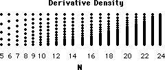
So eventually, a bunch of points becomes a line? No actually, if enough data points are bunched closely enough together they appear as a line. So even though each data point exists separately, independent from the rest, broken up by the days and nights, they appear as a continuous whole, when viewed from a grand enough perspective. They appear to take on a continuous life of their own. It is this continuity that we refer to in the Notebook, Spiral Time.
But as we've seen above, each of the levels is only pretending to be dimensional. Just as the initial points were only pretending to be a line by clustering together, so on each higher level do they pretend to be real by clustering together in vast amounts. What we're pointing out is that each individual derivative is only one number. But they are constructed in the manner shown above. The unfurled Data is a single point.
The Decaying Average is a linear number based upon a line of points. Remember the more points the denser the line. Unfurling a piece of data gives it dimensionality. Unfurling diminishes the individual data, but combines it with the rest of the Data to give it linearity, and its first dimensionality. But remember it is only a logarithmic fractal response, because it is based upon Decay, hence it only achieves partial dimensionality.
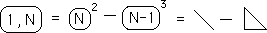
With each unfurling the data achieves another dimension, or at least partial dimensionality. The First Derivative, Directional or Deviational, is the difference between a linear number and a planar number. With each Unraveling comes another Unfurling and another Dimension. All of our Derivatives are based upon differences. The First Derivative is based upon the difference between the present linear fractal response and the most recent planar fractal response.
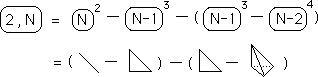
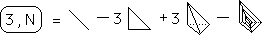
The 2nd Derivative, in Seed Equation terminology, is the difference between two differences: the difference between a linear and planar number and the difference between a planar and a spatial number.
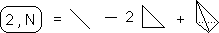
Combining terms, we get a more concise expression. In different terms, the 2nd Directional is equal to the difference between the sum of the linear and spatial dimensions of the data and twice the planar dimension. What does this mean? Who knows? We're just having fun.
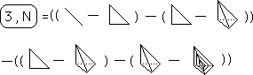
In some ways, each Unraveling or Unfurling gives the Data another dimension. With the 3rd Directional a fourth dimensional response is introduced. First we show the 3rd Directional unfolded in dimensional terminology.
We combine terms to compress the equation and reveal Pascal's Triangle hiding underneath.
We have spoken about the Data as a point, the Decaying Average as a line, the 1st Directional as a plane, and the 2nd Directional as a solid. We could just as easily, maybe more so, have talked about the Data as a scalar line. Then the Decaying Average would be a plane, the 1st Directional a solid, and the 2nd Directional as a 4th dimensional solid. In some ways this would have been easier because our dimensions would have coincided with our Q numbers for Unraveling. When Q = 2, our measure would be constructed in the 2 dimensional plane and then collapsed into a 1 dimensional scalar line for comparison. This coincides with our view of the Decaying Average as constructed by a Spiral Square. Thus this expanded view of the Data as a scalar line rather than a point would have coincided with our geometric understanding of the construction of the measures.
The cube below is the geometrical representation of the 3rd Unraveling, Q=3. When viewed straight on as a square, each rectangle represents the potential impact of a Decaying Average upon the 3rd Unraveling. The largest represents the most recent Decaying Average. As the rectangles spiral in they represent the potential impact of previous Decaying Averages, more and more separated from the most recent. The potential impact of distant Decaying Averages shrinks to almost nothing. From discussions above we also know that each Decaying average can be represented as planar spiral of Data. So each Decaying Average rectangle can be constructed or visualized as dimensional extension into another plane. Remember that the most recent Decaying Average will have the same impact upon the 3rd Unraveling that the most recent Data will have upon the Decaying Average. But while the Data is made up of only one measure, the Decaying Average is made up of all the Data. So the cube below represents the construction of the 3rd unraveling, with each rectangular prism representing the influence of each Data Point. Similarly a tesseract, a 4th Dimensional cube, could be drawn to represent the construction of the 4th Unraveling.
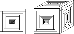
There are no real dimensions associated with our geometrical representations. They only represent the whole Impact. The square represents the whole impact. The cube represents the whole impact. The tesseract represents the whole impact. Each dimension can be collapsed to the dimension before along the lines of Unraveling. A second dimensional 3rd unraveling is equivalent to a 1 dimensional 2nd Unraveling, or a 3rd dimensional 4th unraveling. The above square can be viewed as a 6th Unraveling square with 5th level unraveling rectangles. The cube can be viewed as a 6th level unraveling with 4th level unraveling prisms. The other levels are locked up inside the prisms. We can collapse or expand our structures up and down to understand the basic construction of each Raveling measure. So whether we view the Data as points or scalar lines makes no difference. The Data as a point made more sense when exploring the number of terms making up a Raveling, because each piece of Data represented only one term. Viewing the Data as a line makes more sense when speaking about its impact as a scalar measure. It is irrelevant which view is taken because of the collapsibility of the dimensions in this scheme.